Let’s talk about the progress we’ve made on a kD-Tree decomposition.
Hi all,
Matt just set up this blog to document some of the developments that are going on in yt, and he asked me to share some of the work we’ve recently done on a kD-Tree decomposition primarily used for the volume rendering, so here goes.
This semester I took a High Performance Scientific Computing course here at Boulder where a large fraction of our work revolved around a final project. Luckily for me, I was able to work on a new parallel decomposition framework for the volume renderer inside yt. What resulted was primarily a kD-tree decomposition of our AMR datasets. While kD-tree are usually used to organize point-like objects, we modified it to separate regions of space.
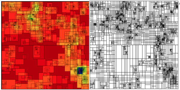
Our kD-tree has 2 primary objects: dividing nodes and leaf nodes. Each dividing node has a position, a splitting axis, and pointers to left and right children. The children are then either additional dividing nodes or leaf nodes. The dividing nodes therefore recursively split up the domain until the ‘bottom’ is composed of all leaf nodes. Each leaf node represents a brick of data that has the same resolution and is covered by a single AMR grid. A leaf doesn’t have to (and rarely does) encompass an entire grid. A leaf contains various information such as what AMR grid it resides in, what the start and end indices are in that grid, the estimated cost to render the leaf, and the left and right corners of the space it covers.
So what does this do for us? Well, the kD-Tree decomposition allows a unique back-to-front ordering of all the data. This ordering is determined on the fly by comparing the viewpoint with the dividing node position and splitting axis. By comparing these two, we are able to navigate all the way to the ‘back’ of the data and recursively step through the data. This decomposition also provides at least 2 different ways of load-balancing the rendering. By estimating the cost of each leaf, we can subdivide the back-to-front ordering of grids into Nprocs chunks and have each processor only work on their part. This subdivision is viewpoint-dependent such that the first processor always gets the furthest 1/Nth of the data. This subdivision is done on each processor and no communication between them is needed. The second method to implement a ‘breadth-first’ traversal of the tree where we first create Nprocs sub-trees that are not as well load balanced as the first method but are viewpoint-independent. Each processor is then handed one of the sub-trees to completely render. This time, when the viewpoint changes, the regions that each processor ‘owns’ stays the same.
Now one important part in both of these methods is how we composite the individual images back into a single image. This has been studied a bunch in image processing and is what I think is known as an ‘over-operation’. For us, all this means is that we combine each pair of images using their alpha channels correctly to blend the images together. This is essentially the same operation that is done during the actual ray-casting. This composition is simple for the first decomposition method because we know exactly which order each processor’s image goes in, and construct a binary tree reduction onto the root processor. In the second case where there is a more arbitrary ordering of each of the images, we use the same knowledge from the kD-Tree to combine each pair of images in the correct order. For now, this implementation is living in the kd-render branch of the yt mercurial repository, but I imagine that after some more testing and trimming it will make its way back into the main trunk. If you are interested in using it, you mainly have to change two calls in the rendering:
When instantiating the volume rendering, you need to add the kd=True
and pf=pf keywords.
vp = pf.h.volume_rendering(L, W, c, (SIZE,SIZE), planck,
         fields=['Temperature', 'RelativeDensity'],
         pf=pf, kd=True, l_max=None,
         memory_factor=0.5)
Then, instead of vp.ray_cast() we use either the back-to-front
partitioning:
vp.kd_ray_cast(memory_per_process=2**30) # 1GB per processor
or the breadth first:
vp.kd_breadth_ray_cast(memory_per_process=2**30) # 1GB per processor
There are two additional keywords shown above that somewhat useful for large datasets. Because there can be several leafs that use the same vertex-centered-data of a single grid, it is important to save as much of that information in memory so that disk I/O doesn’t hinder the performance. To do this, we’ve implemented a rudimentary cacheing system that stores as much of the vertex centered data as possible. The memory_factor keyword lets us know what fraction of the memory per processor to use, and memory_per_process tells us how much memory each processor has access to. This is fairly experimental and if you run out of memory, I’d suggest cutting one of these two options by a factor of 5-10.
Anyways, that’s about it for the discussion of the new kD-Tree decomposition for volume rendering. As we make improvements some of this may change, so keep an eye out for those. Let me just mention that this isn’t the only thing this kD-Tree can be used for, so if you have any thoughts or questions, feel free to email me (sam.skillman@gmail.com) or perhaps comment on this post.
Cheers, Sam