This post shows how to generate particle fields from pre-defined particle lists, lattice distributions, and distributions based on density fields.
Particle Generators
Generating particle initial conditions is now possible in yt. The following shows how to generate particle fields from pre-defined particle lists, lattice distributions, and distributions based on density fields.
First, we define a gridded density field where the particle density field has been “cloud-in-cell” (CIC) interpolated to the grid, and define a function that assigns a set of particle indices based on a number of particles and a starting index. This is for a case where we want to add particles to an already existing set but make sure they have uniqune indices.
In[1]:
    from yt.mods import *
    from yt.utilities.particle_generator import *
    import yt.utilities.initial_conditions as ic
    import yt.utilities.flagging_methods as fm
    from yt.frontends.stream.api import refine_amr
    from yt.utilities.lib import CICDeposit_3

    def _pgdensity(field, data):
        blank = np.zeros(data.ActiveDimensions, dtype='float32')
        if data.NumberOfParticles == 0: return blank
        CICDeposit_3(data["particle_position_x"].astype(np.float64),
                     data["particle_position_y"].astype(np.float64),
                     data["particle_position_z"].astype(np.float64),
                     data["particle_gas_density"].astype(np.float32),
                     np.int64(data.NumberOfParticles),
                     blank, np.array(data.LeftEdge).astype(np.float64),
                     np.array(data.ActiveDimensions).astype(np.int32),
                     np.float64(data['dx']))
        return blank
    add_field("particle_density_cic", function=_pgdensity,
              validators=[ValidateGridType()],
              display_name=r"$\mathrm{Particle}\/\mathrm{Density}$")

    def add_indices(npart, start_num) :
        return np.arange((npart)) + start_num
Next, we’ll set up a uniform grid with some random density data:
In[2]:
    domain_dims = (128, 128, 128)
    dens = 0.1*np.random.random(domain_dims)
    fields = {"Density": dens}
    ug = load_uniform_grid(fields, domain_dims, 1.0)
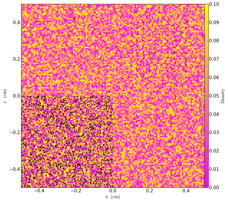
As a first example, we’ll generate particle fields from pre-existing NumPy arrays. First, we define a list of particle field names, and then assign random positions to the particles in one corner of the grid. We then call FromListParticleGenerator, which generates the particles. assign_indices assigns the indices (using numpy.arange by default). apply_to_stream applies the particle fields to the grid.
In[3]:
    num_particles1 = 10000
    field_list = ["particle_position_x","particle_position_y",
                  "particle_position_z","particle_gas_density"]
    x = np.random.uniform(low=0.0, high=0.5, size=num_particles1) # random positions
    y = np.random.uniform(low=0.0, high=0.5, size=num_particles1) # random positions
    z = np.random.uniform(low=0.0, high=0.5, size=num_particles1) # random positions
    pdata = {'particle_position_x':x,
             'particle_position_y':y,
             'particle_position_z':z}
    particles1 = FromListParticleGenerator(ug, num_particles1, pdata)
    particles1.assign_indices()
    particles1.apply_to_stream()
    yt : [INFO     ] 2013-01-01 21:24:32,484 Adding Density to list of fields
    yt : [INFO     ] 2013-01-01 21:24:32,486 Adding particle_position_z to list of fields
    yt : [INFO     ] 2013-01-01 21:24:32,487 Adding particle_index to list of fields
    yt : [INFO     ] 2013-01-01 21:24:32,487 Adding particle_position_x to list of fields
    yt : [INFO     ] 2013-01-01 21:24:32,488 Adding particle_position_y to list of fields
Now that the particles are part of the parameter file, they may be manipulated and plotted:
In[4]:
    slc = SlicePlot(ug, 2, ["Density"], center=ug.domain_center)
    slc.set_cmap("Density","spring")
    slc.annotate_particles(0.2, p_size=10.0) # Display all particles within a thick slab 0.2 times the domain width
    slc.show()

Now let’s try adding a particle distribution in a lattice-shaped spatial arrangement. Let’s choose ten particles on a side, and place them in a small region away from the random particles. We’ll use the special add_indices function we defined earlier to assign indices that are all different from the ones the already existing particles have.
In[5]:
    pdims = np.array([10,10,10]) # number of particles on a side in each dimension
    ple = np.array([0.6,0.6,0.6]) # left edge of particle positions
    pre = np.array([0.9,0.9,0.9]) # right edge of particle positions
    particles2 = LatticeParticleGenerator(ug, pdims, ple, pre, field_list)
    particles2.assign_indices(function=add_indices, npart=np.product(pdims),
                              start_num=num_particles1)
    particles2.apply_to_stream()
yt : [INFO ] 2013-01-01 21:24:33,957 Adding particle_gas_density to list of fields
We now have both sets of particles:
In[6]:
    slc = SlicePlot(ug, 2, ["Density"], center=ug.domain_center)
    slc.set_cmap("Density","spring")
    slc.annotate_particles(0.2, p_size=10.0)
    slc.show()

And by sorting all of the indices we can check that all of them are unique, as advertised:
In[7]:
    dd = ug.h.all_data()
    indices = np.sort(np.int32(dd["particle_index"]))
    print "All indices unique = ", np.all(np.unique(indices) == indices)
All indices unique = True
Now let’s get fancy. We will use the initial conditions capabilities of yt to apply a spherically symmetric density distribution based on the “beta-model” functional form, and set up a refinement method based on overdensity. Then, we will call refine_amr to apply this density distribution and refine the grid based on the overdensity over some value.
In[8]:
    fo = [ic.BetaModelSphere(1.0,0.1,0.5,[0.5,0.5,0.5],{"Density":(10.0)})]
    rc = [fm.flagging_method_registry["overdensity"](4.0)]
    pf = refine_amr(ug, rc, fo, 3)
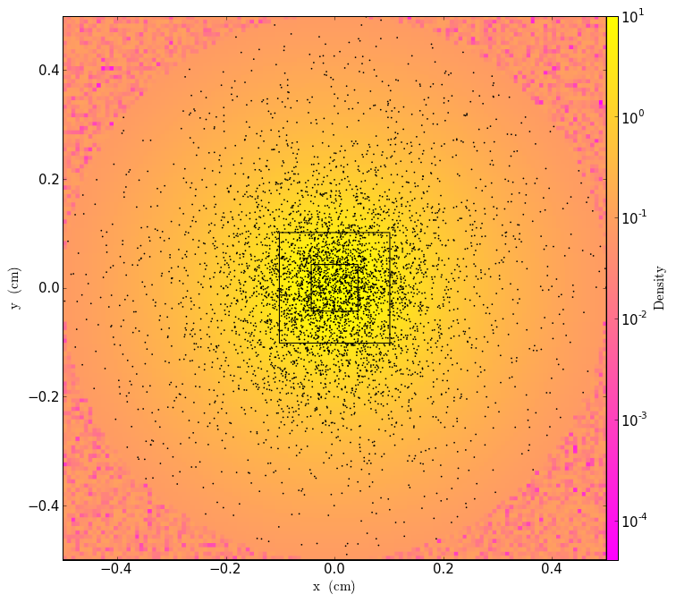
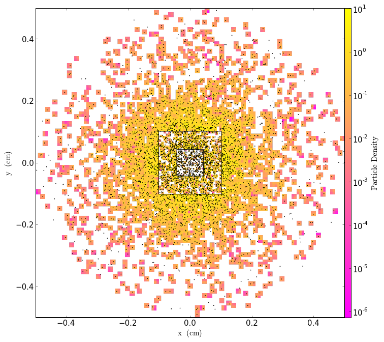
Now, we have an interesting density field to serve as a distribution function for particle positions. What we do next is define a spherical region over which particle positions will be generated based on the local grid density. We also will map the grid density to a particle density field using cloud-in-cell interpolation. Finally, when we apply these particles, we will set the optional argument clobber=True, which will remove the particles we already created.
In[9]:
    num_particles3 = 100000
    map_dict = {"Density": "particle_gas_density"} # key is grid field, value is particle field
    sphere = pf.h.sphere(pf.domain_center, (0.5, "unitary"))
    particles3 = WithDensityParticleGenerator(pf, sphere, num_particles3,
                                              field_list)
    particles3.assign_indices()
    particles3.map_grid_fields_to_particles(map_dict) # Map density fields to particle fields
    particles3.apply_to_stream(clobber=True) # Get rid of all pre-existing particles
Now we’ll plot up both the grid density field and the “particle_density_cic” field (defined at the top of the script), which is mapped from the particles onto the grid. We also overplot the particle positions. These should roughly correspond to the non-zero values of “particle_density_cic”, but there will be some discrepancies due to the fact that they are taken from a thick slab and only a slice of the grid-based field is shown.
In[10]:
    slc = SlicePlot(pf, 2, ["Density","particle_density_cic"], center=pf.domain_center)
    slc.set_log("Density", True)
    slc.set_log("particle_density_cic", True)
    slc.set_cmap("all", "spring")
    slc.annotate_grids()
    slc.annotate_particles(0.01,p_size=3)
    slc.show()


