How to export surfaces into an obj file (will it blend?!)
OBJ File Exporter for Surfaces
OBJ and MTL Files
If the ability to maneuver around an isosurface of your 3D simulation in
Sketchfab cost you half a day of work (let’s be
honest, 2 days), prepare to be even less productive. With a new
OBJ file
exporter, you can now
upload multiple surfaces of different transparencies in the same file.
The following code snippet produces two files which contain the vertex info
(surfaces.obj) and color/transparency info (surfaces.mtl) for a 3D
galaxy simulation:
   from yt.mods import *

   pf = load("/data/workshop2012/IsolatedGalaxy/galaxy0030/galaxy0030")
   rho = [2e-27, 1e-27]
   trans = [1.0, 0.5]
   filename = './surfaces'

   sphere = pf.h.sphere("max", (1.0, "mpc"))
   for i,r in enumerate(rho):
       surf = pf.h.surface(sphere, 'Density', r)
       surf.export_obj(filename, transparency = trans[i], color_field='Temperature', plot_index = i)
The calling sequence is fairly similar to the export_ply function
previously used
to export 3D surfaces. However, one can now specify a transparency for each
surface of interest, and each surface is enumerated in the OBJ files with plot_index.
This means one could potentially add surfaces to a previously
created file by setting plot_index to the number of previously written
surfaces.
One tricky thing: the header of the OBJ file points to the MTL file (with
the header command mtllib). This means if you move one or both of the files
you may have to change the header to reflect their new directory location.
A Few More Options
There are a few extra inputs for formatting the surface files you may want to use.
(1) Setting dist_fac will divide all the vertex coordinates by this factor.
Default will scale the vertices by the physical bounds of your sphere.
(2) Setting color_field_max and/or color_field_min will scale the colors
of all surfaces between this min and max. Default is to scale the colors of each
surface to their own min and max values.
Uploading to SketchFab
To upload to Sketchfab one only needs to zip the OBJ and MTL files together, and then upload via your dashboard prompts in the usual way. For example, the above script produces this beautiful rendering
Importing to MeshLab and Blender
The new OBJ formatting will produce multi-colored surfaces in both MeshLab and Blender, a feature not possible with the previous PLY exporter. To see colors in MeshLab go to the “Render” tab and select “Color -> Per Face”. Note in both MeshLab and Blender, unlike Sketchfab, you can’t see transparencies until you render.
…One More Option
If you’ve started poking around the actual code instead of skipping off to lose a few days running around your own simulations you may have noticed there are a few more options then those listed above, specifically, a few related to something called “Emissivity.” This allows you to output one more type of variable on your surfaces. For example:
   from yt.mods import *

   pf = load("/data/workshop2012/IsolatedGalaxy/galaxy0030/galaxy0030")
   rho = [2e-27, 1e-27]
   trans = [1.0, 0.5]
   filename = './surfaces'

   def _Emissivity(field, data):
       return (data['Density']*data['Density']*np.sqrt(data['Temperature']))
   add_field("Emissivity", function=_Emissivity, units=r"\rm{g K}/\rm{cm}^{6}")

   sphere = pf.h.sphere("max", (1.0, "mpc"))
   for i,r in enumerate(rho):
       surf = pf.h.surface(sphere, 'Density', r)
       surf.export_obj(filename, transparency = trans[i],
                       color_field='Temperature', emit_field = 'Emissivity',
		       plot_index = i)
will output the same OBJ and MTL as in our previous example, but it will scale an emissivity parameter by our new field. Technically, this makes our outputs not really OBJ files at all, but a new sort of hybrid file, however we needn’t worry too much about that for now.
This parameter is useful if you want to upload your files in Blender and have the embedded rendering engine do some approximate ray-tracing on your transparencies and emissivities. This does take some slight modifications to the OBJ importer scripts in Blender. For example, on a Mac, you would modify the file “/Applications/Blender/blender.app/Contents/MacOS/2.65/scripts/addons/io_scene_obj/import_obj.py”, in the function “create_materials” with:
                    elif line_lower.startswith(b'tr'):  # translucency
                        context_material.translucency = float_func(line_split[1])
                    elif line_lower.startswith(b'tf'):
                        # rgb, filter color, blender has no support for this.
                        pass
                    elif line_lower.startswith(b'em'): # MODIFY: ADD THIS LINE
                        context_material.emit = float_func(line_split[1]) # MODIFY: THIS LINE TOO
                    elif line_lower.startswith(b'illum'):
                        illum = int(line_split[1])
To use this in Blender, you might create a Blender script like the following:
   import bpy
   from math import *

   bpy.ops.import_scene.obj(filepath='./surfaces.obj') # will use new importer

   # set up lighting = indirect
   bpy.data.worlds['World'].light_settings.use_indirect_light = True
   bpy.data.worlds['World'].horizon_color = [0.0, 0.0, 0.0] # background = black
   # have to use approximate, not ray tracing for emitting objects ...
   #   ... for now...
   bpy.data.worlds['World'].light_settings.gather_method = 'APPROXIMATE'
   bpy.data.worlds['World'].light_settings.indirect_factor=20. # turn up all emiss

   # set up camera to be on -x axis, facing toward your object
   scene = bpy.data.scenes["Scene"]
   scene.camera.location = [-0.12, 0.0, 0.0] # location
   scene.camera.rotation_euler = [radians(90.), 0.0, radians(-90.)] # face to (0,0,0)

   # render
   scene.render.filepath ='/Users/jillnaiman/surfaces_blender' # needs full path
   bpy.ops.render.render(write_still=True)
This above bit of code would produce an image like so:
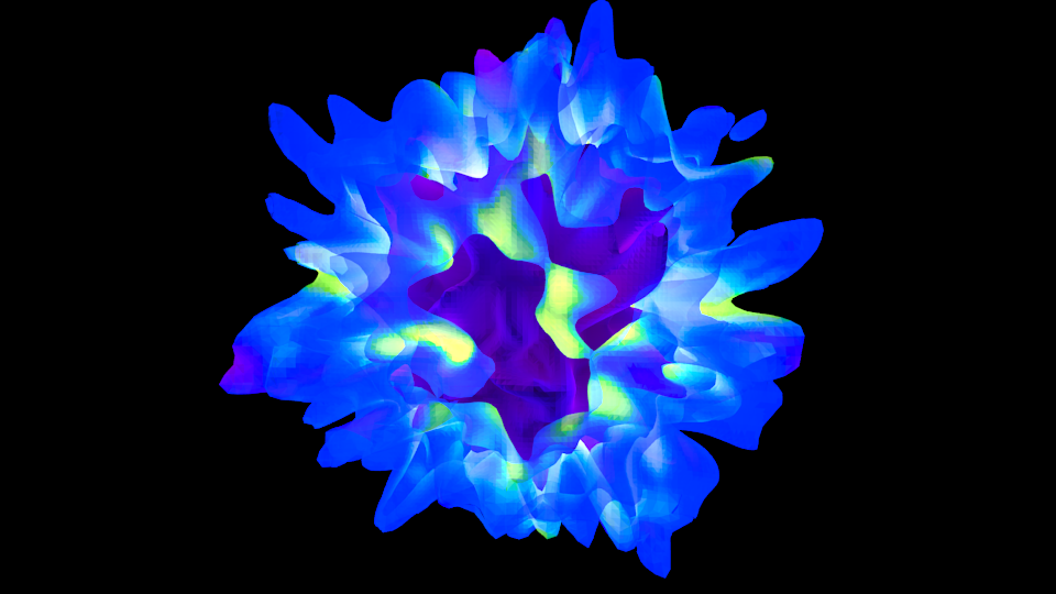
Our cool image
Note that the hottest stuff is brightly shining, while the cool stuff is less so (making the inner isodensity contour barely visible from the outside of the surfaces).
If the Blender image caught your fancy, you’ll be happy to know there is a greater integration of Blender and yt in the works, so stay tuned!